An R package for spatially-constrained clustering using either distance or covariance matrices. “Spatially-constrained” means that the data from which clusters are to be formed also map on to spatial coordinates, and the constraint is that clusters must be spatially contiguous.
The package includes both an implementation of the REDCAP collection of efficient yet approximate algorithms described in D. Guo’s 2008 paper, “Regionalization with dynamically constrained agglomerative clustering and partitioning.” (pdf available here), with extension to covariance matrices, and a new technique for computing clusters using complete data sets. The package is also designed to analyse matrices of spatial interactions (counts, densities) between sets of origin and destination points. The spatial structure of interaction matrices is able to be statistically analysed to yield both global statistics for the overall spatial structure, and local statistics for individual clusters.
Installation
The easiest way to install spatialcluster is be enabling the corresponding r-universe:
options (repos = c (
    mpadge = "https://mpadge.r-universe.dev",
    CRAN = "https://cloud.r-project.org"
))
The package can then be installed as usual with,
install.packges ("spatialcluster")Alternatively, the package can also be installed using any of the following options:
# install.packages("remotes")
remotes::install_git ("https://codeberg.org/mpadge/spatialcluster")
remotes::install_git ("https://git.sr.ht/~mpadge/spatialcluster")
remotes::install_bitbucket ("mpadge/spatialcluster")
remotes::install_gitlab ("mpadge/spatialcluster")
remotes::install_github ("mpadge/spatialcluster")
Usage
The two main functions, scl_redcap() and scl_full(), implement different algorithms for spatial clustering. The former implements the REDCAP collection of efficient yet approximate algorithms described in D. Guo’s 2008 paper, “Regionalization with dynamically constrained agglomerative clustering and partitioning.” (pdf available here), with extension here to apply clustering to covariance matrices. These algorithms are computationally efficient yet generate only approximate estimates of underlying clusters. The second function, scl_full(), trades computational efficiency for accuracy, through generating clustering schemes using all available data.
In short:
-
scl_full()should always be preferred as long as it returns results within a reasonable amount of time -
scl_redcap()should be used only where data are too large forscl_full()to be run in a reasonable time.
For clustering a group of n points, both of these functions require three main arguments:
- A rectangular matrix of spatial coordinates of points to be clustered (
nrows; at least 2 columns); - An
n-by-nsquare matrix quantifying relationships between those points; - A single value (
ncl) specifying the desired number of clusters.
The following code demonstrates usage with randomly-generated data:
The load the package and call the function:
library (spatialcluster)
scl <- scl_full (xy, dmat, ncl = 8)
plot (scl)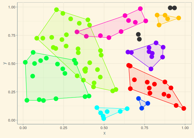
Both functions return a list with the following components:
names (scl)
#> [1] "tree"       "merges"     "ord"        "nodes"      "pars"
#> [6] "statistics"-
treedetails distances and cluster numbers for all pairwise comparisons between objects. -
mergesdetails increasing distances at which each pair of objects was merged into a single cluster. -
ordprovides the order of the merges (forscl_full()only). -
nodesrecords the spatial coordinates of each point (node) of the input data. -
parsretains the parameters used to call the clustering function. -
statsiticsreturns the clustering statistics, both for individual clusters and an overall global statistic for the clustering scheme as a whole.
See the “Get Started” vignette for more details.
A Cautionary Note
The following plot compares the results of applying four different clustering algorithms to the same data.
library (ggplot2)
library (gridExtra)
scl <- scl_full (xy, dmat, ncl = 8, linkage = "single")
p1 <- plot (scl) + ggtitle ("full-single")
scl <- scl_redcap (xy, dmat, ncl = 8, linkage = "single")
p2 <- plot (scl) + ggtitle ("redcap-single")
scl <- scl_redcap (xy, dmat, ncl = 8, linkage = "average")
p3 <- plot (scl) + ggtitle ("redcap-average")
scl <- scl_redcap (xy, dmat, ncl = 8, linkage = "complete")
p4 <- plot (scl) + ggtitle ("redcap-complete")

grid.arrange (p1, p2, p3, p4, ncol = 2)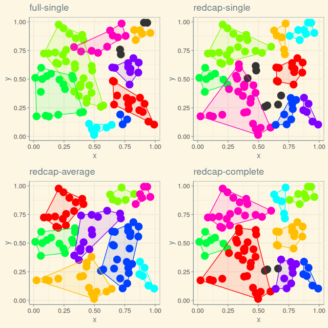
This example illustrates the universal danger in all clustering algorithms: they can not fail to produce results, even when the data fed to them are definitely devoid of any information as in this example. Clustering algorithms should only be applied to reflect a very specific hypothesis for why data should be clustered in the first place; spatial clustering algorithms should only be applied to reflect two very specific hypothesis for (i) why data should be clustered at all, and (ii) why those clusters should manifest a spatial pattern.
