Introduction
spatialcluster is an R package for
performing spatially-constrained clustering. Spatially-constrained
clustering is a distinct mode of clustering in which data include
additional spatial coordinates in addition to the data used for
clustering, and the clustering is performed such that only spatially
contiguous or adjacent points may be merged into the same cluster (Fig.
1).
Nomenclature
- The term “objects” is used here to refer to the objects which are to be aggregated into clusters; these may be points, lines, polygons, or any other spatial or non-spatial entities
- The term “non-spatial data” also encompasses data which are not necessarily spatial, but which may include some spatial component.
Distance-based versus covariance-based clustering
Almost all clustering routines have been developed for application to distance matrices. Distance-based clustering algorithms generally seek to aggregate objects into clusters that maximise the homogeneity of distances between points in each cluster. Clustering may also be performed on covariance or correlation matrices. The object of clustering covariance matrices is to maximise intra-cluster covariance while minimising inter-cluster covariance.
Both the SKATER and REDCAP algorithms, for example, utilise as a measure of inter-cluster homogeneity the sums of squared deviations from mean values. The equivalent measure for covariance-based clustering is simply the sum of covariances. The present approach to covariance clustering extends beyond techniques generally considered under the term “correlation clustering”. Correlation clustering is often applied in cases where an observation and reference matrix are available, with clusters defined as simply those groups for which observed correlations exceed reference correlations. The present approach also uses observation and reference matrices, yet extends beyond traditional correlation clustering through tracing the subsequent hierarchy of merges of all clusters. This is particularly important in spatially-constrained clustering, for which simple correlation clustering techniques are often not applicable, as they result in large numbers of very small clusters, with no way to merge those into larger clusters.
The software accompanying this manuscript has been developed to accept both distance and covariance matrices as input. It includes a reference implementation of the REDCAP algorithms adapted as described below for clustering covariance matrices.
Observation and reference matrices for covariance clustering
The present work is focussed on spatially-constrained clustering based on non-spatial data representing objects which also have spatial locations. “Spatially-constrained” implies that the clusters are constrained to be spatially contiguous. Spatial data that involve counts or densities are often represented in terms of flow matrices or, in conventional studies of human transport system, “origin-destination” matrices. Such matrices are rectangular, and represent tallies of numbers, densities, or, in general terms, flows between a set of origins and a (possibly different) set of destinations.
Such flow data can - and indeed often are - directly submitted to clustering routines, through constructing some suitably-scaled metric of distance as the inverse of flow. In spatial systems, however, flows from some point to another point are often closely related to flows from some point near to some near , with similarity positively related to the proximity of to and to . This is nothing other than a definition of “autocorrelation”. (It is also implicitly tautological, as are most definitions of this phenomenon.) Clustering with directly observed flows alone ignores the effects of autocorrelation, and thus introduces a host of well-recognised issues arising through doing so.
Flow matrices may be converted into covariance matrices through populating the upper or lower triangle with pair-wise covariances (or through copying one triangle to the other to generate a symmetrical covariance matrix). Covariances can be calculated between the rows of a flow matrix to yield covariances in flows from each point, or between the columns to yield covariances in flows to each point. Of course, both may be combined through, for example, filling the upper triangle of a covariance matrix with row-wise covariances, and the lower triangle with column-wise covariances. The value will then represent the covariance in flow from i and flow from j, while will represent the covariance in flow to i and flow to j. Such compound covariance matrices will not be symmetrical.
Both forms of population covariance matrices are explicitly demonstrated in the empirical application below, revealing the usefulness of considering and comparing both forms of covariance matrices. Values of covariance will manifest similar properties to raw flows, in that nearby values are likely to be more similar or “autocorrelated.” For many spatial processes, “neutral” models of flows have been developed, and can be applied to yield estimates of covariances expected in the presence of these kinds of processes alone. Such estimated covariance matrices are the “reference” matrices referred to above, and are generated in the present work through applying spatial interaction models to the observed flow data, and generating corresponding covariance matrices. These matrices effectively represent the covariance expected in the presence of a particular type of autocorrelation. The difference with observed covariance matrices may then be interpreted to reflect the effects of processes beyond spatial autocorrelation.
Observation and reference matrices for correlation clustering
The ability to calculate observation and reference covariance matrices enables a standardised covariance matrix to be generated, in which positive values represent values of covariance beyond those expected on the basis of the neutral model alone (here, a spatial interaction model). Note, moreover, than negative values may also be interpreted in the observe way: to reflect spatial clusters in which flows are significantly less likely than those expected on the basis of a neutral model alone. The methods developed below are applied separately to positive and negative values of the net covariance matrix, with clusters only formed from either exclusively positive or exclusively negative values. Covariances in such clusters will thus always be entirely significant in the sense of T-tests for divergence from expected values of zero. Thus by definition, any clusters discerned by the methodology may be presumed entirely significant. The software produces summary statistics for each cluster (T- and p-values), enabling the relative significance of different clusters to be compared.
Note that it will not generally be possible - absent specific hypotheses - to provide a global statistic quantifying the significance of a clustering scheme. This is primarily because there is no reason to presume that positive net covariances will be more likely to form distinct clusters than will negative net covariances. The overall distribution of net covariances will thus generally be symmetrical, although it may also be asymmetrical when spatial patterns of positive net covariance differ from those of negative net covariance - for example through positive covariances being very strongly concentrated in a small number of clusters, while negative covariances remain more dispersed.
Spatial clustering versus spatially-constrained clustering
Spatial clustering
Spatial clustering is a very well-studied field (see reviews in Han, Kamber, and Tung 2001; Duque, Ramos, and Suriñach 2007; Lu 2009), with many methods implemented in the R language (see the CRAN Task View on Analysis of Spatial Data). Spatial clustering algorithms take as input a set of spatial distances between objects, and seek to cluster those objects based on these exclusively spatial distances alone (Fig. 1A). Other non-spatial data may be included, but must be somehow reconciled with the spatial component. This is often achieved through weighted addition to attain approximately “spatialized” data. Figure 1B-C illustrate two related non-spatial (B) and spatial (C) datasets. The primary data of interest depicted in B can be “spatialized” through additively combining the associated distance matrices of non-spatial and spatial data, and submitting the resultant distance matrix to a clustering routine of choice.
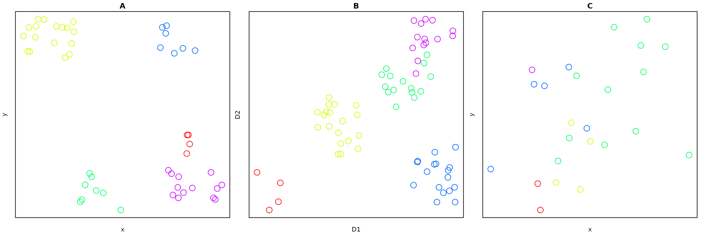
Figure 1: (A) Illustration of typical spatial clustering application for which input data are explicit spatial distances between points; (B) Illustration of clustering in some other, non-spatial dimensions, D1 and D2, for which associated spatial data in (C) do not manifest clear spatial clusters.
For example, the following code illustrates the use of the
DBSCAN algorithm (Density
Based Spatial
Clustering of Applications with
Noise) from the R package dbscan.
d_nospace <- dist (dat_nospace) # matrix of non-spatial data
d_space <- dist (dat_space) # 2-column matrix of spatial data
d <- dat_nospace + d_space # simple linear addition##
## Attaching package: 'dbscan'## The following object is masked from 'package:stats':
##
## as.dendrogram
db <- dbscan::dbscan (d, eps = 0.4) # more on the eps parameter below
db
## DBSCAN clustering for 49 objects.
## Parameters: eps = 0.4, minPts = 5
## Using euclidean distances and borderpoints = TRUE
## The clustering contains 4 cluster(s) and 4 noise points.
##
## 0 1 2 3 4
## 4 17 9 7 12
##
## Available fields: cluster, eps, minPts, metric, borderPoints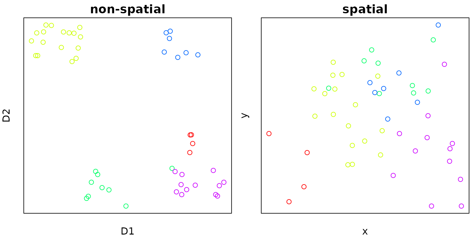
Figure 2: (A) Non-spatial data coloured by dbscan clustering results; (B) Corresponding spatial data coloured by dbscan clustering results.
These results demonstrate that reasonable results can indeed be
obtained through simple linear combination of non-spatial and spatial
distances. This approach is very simple, and it is very easy to submit
such combined distance matrices to high-performance clustering routines
such as dbscan.
There are nevertheless two notable shortcomings:
- There is no objectively best way to combine non-spatial and spatial distance matrices; and
- Routines such as
dbscanstill require an effectively arbitrary parameter represented by the above value ofeps = 0.4. This value was simply chosen to best reflect the known structure of the input clusters, but in any practical application will remain largely arbitrary.
Even one of the most recent R packages dedicated to spatial clustering (Chavent et al. 2017) follows precisely this linear addition strategy, via a parameter determining the relative weights of the non-spatial and spatial data.
We assert here that such approaches provide more a means of attaining approximately spatially-structured clustering schemes, rather than actually providing spatially-constrained clusters in the sense we now explore.
Spatially-constrained clustering
The spatialcluster
package performs strict spatially constrained clustering.
This means that clusters are formed entirely on the basis of the
non-spatial data, while the spatial data provide a constraint used to
ensure that all clusters are spatially contiguous.
The SKATER algorithm
One of the most widespread algorithms for spatially constrained
clustering is the so-called “SKATER” algorithm (Spatial Kluster
Analysis by Tree Edge
Removal, AssunÇão et al. 2006), available via
the R package spdep
(Bivand, Hauke, and Kossowski 2013; Bivand and
Piras 2015). This algorithm constructs a minimum spanning tree
(MST) connecting neighbours defined by the spatial data, with all
connections defined by minimal distances in the non-spatial data. The
SKATER algorithm constructs the simplest of all MSTs, by iterating
through the list of neighbouring edges according to increasing
(non-spatial) distance, and inserting edges where these connect
previously unconnected objects. The resultant MST is then partitioned
into a specified number of clusters such that the intra-cluster sum of
squared deviations from the mean (of the non-spatial data) is minimised.
Further details are given in AssunÇão et al.
(2006).
The REDCAP algorithms
The REDCAP algorithms for spatially-constrained clustering (REgionalization with Dynamically Constrained Agglomerative Clustering, Guo 2008) employs three distinct methods for constructing MSTs. The original algorithms actually develop these three methods for two distinct ways of constructing spanning trees: through using nearest neighbours only (“first-order constraint”), or through considering all neighbours of each object (“full-order constraint”). The results of the cited manuscript clearly reveal the superiority of the latter, and only full-order constraints are considered here.
The three methods refer to methods for determining which edges are selected to link clusters, via either single-, average-, or complete-linkage, which function as follows:
- Single-linkage clustering simply loops through the list of minimal-distance, nearest-neighbour edges, and inserts each next-minima distance edge into the clustering tree if it is not part of any previous cluster, and if it connects two separate yet contiguous clusters.
- Average-linkage clustering assigns weights to each unassigned edge based on their average distance to all edges within all adjacent clusters. Thus when an edge becomes part of a cluster, the distances to all non-assigned edges adjacent to that cluster are updated to reflect the change in average distance calculated over all edges in that cluster. Edges are continually (re-)sorted based on average distances, and the tree is built through sequentially inserting minimal-distance edges.
- Maximal-linkage clustering forms clusters through inserting the edge having the minimal distance to the farthest point of any adjacent cluster.
Single-linkage is equivalent to the SKATER algorithm, where the single best edge connecting two clusters is selected. (The SKATER algorithm is actually equivalent to the worst-performing REDCAP algorithm: single-linkage, first-order constraint.) (See Guo 2008 for details.) The resultant MSTs are then partitioned into specified numbers of clusters using an identical approach to SKATER, namely through minimising the intra-cluster sum of squared deviations from mean values.
The REDCAP algorithms and covariance clustering
The software accompanying this manuscript includes a reference implementation of the REDCAP algorithms (Gu2008?) for distance-based clustering. Conversion of the three algorithms described above to covariance based clustering is straightforward. The first stage of constructing MSTs via the three forms of linkage remains largely identical, with minimal distances simply replaced by maximal covariances. Tree bi-section becomes a slightly different, and computationally simpler, procedure, replacing the previous measure of intra-cluster homogeneity () with a simple maximum (). Application to the two forms of matrix remains otherwise identical.
The Exact Clustering Algorithm
As described above, the REDCAP algorithms provide different ways of constructing minimal spanning trees for a given data set, with resultant clusters based on bisecting these spanning trees. They effectively represent the relationships within a data set by the “best” minimal set (according to the chosen algorithm). Here, we develop a simple algorithm for deriving a clustering scheme that uses the full set of nearest-neighbour relationships in a given data set.
Each point or object within a typical planar (effectively two-dimensional) data set may have on average just under three nearest neighbours if these are calculated with a triangulation, or potentially up to for some -nearest neighbours scheme. Each point in a minimal-spanning tree generally has an average of between two and three neighbours (one for terminal nodes; two for non-branching nodes; three for branching nodes). It may accordingly be presumed that reducing a full set of neighbours to an MST reduces average numbers of edges per node from to . The loss in computational complexity produced through using all neighbouring nodes instead of an MST is thus likely to be only around 20%. Moreover, if a clustering algorithm scales sub-linearly with , as many do, this loss is likely to be even less pronounced with increasing .
The exact clustering algorithm proceeds through the following steps,
looping until all data objects have been allocated to a cluster, and
beginning with both i = 0 and clnum = 0. The
primary data is an array of edges (edge) sorted by
increasing distance.
1.  Select edge [i] connecting nodes a and b.
2.  i++
3.  if both a and b are already in clusters:
        continue to next iteration
    else if neither node is in a cluster:
        cluster (clnum) = create_new_cluster (c (a, b))
        clnum++
    else if only a is in a cluster:
        set_cluster_number (a, get_cluster_number (b))
    else if only b is in a cluster:
        set_cluster_number (b, get_cluster_number (a))
This procedure allocates all nodes (data objects) to clusters. The number of resultant clusters can not be known in advance, and many clusters may be very small, comprising for example only a single edge connecting two nodes. This initial clustering may then be used as the basis of a further hierarchical clustering, through sequentially merging clusters having the minimal distance according to some specified metric. This merging involves linking previously distinct clusters according to some specified criteria, for which the same three criteria used in the REDCAP algorithms can be directly applied here. Note, however, that average and maximal distances in the REDCAP algorithms simply represent the respective average and maximal individual edge distances, and not the corresponding distances traversed within a cluster through the MST.
It is possible within the present exact clustering approach to select edges based on actual average or maximal traversal distances from a potential connecting edge to all other edges in two clusters. Doing so, however, simply merges the two smallest clusters, all other things being equal, because these must by definition have the shortest average and maximal distance. Edge selection is therefore implemented here in the same way as the REDCAP algorithms, by selecting edges based on average and maximal single edge distances. Clusters are hierarchically connected by selecting edges according to on of the following three schemes:
- Single-linkage: select the single edge having the minimal distance between any two clusters;
- Average-linkage: select the edge connecting the two clusters which, when merged, give the lowest average intra-cluster edge distance; or
- Maximal-linkage: select the edge connecting the two clusters which, when merged, gives the lowest maximal intra-cluster edge distance.
The latter two of these yield clusters with preferentially shorter intra-cluster distances, yet the selection procedure remains statistically unbiased by cluster size.
Clustering Origin-Destination (OD) matrices
The exact clustering scheme provides a uniquely powerful approach to discerning spatial clusters in Origin-Destination (OD) matrices. These are ubiquitous in transport planning, and quantify numbers or densities of journeys undertaken between a set of origin points and a (potentially different) set of destination points. Origin-destination matrices are frequently modelled by spatial interaction models, which explain the “interaction” between two locations based on their size, measured as aggregate numbers or densities of trips to and from those points, and their distance apart. The sizes of origin locations are the row sums of the OD matrix; the sizes of destinations the column sums. Respectively denoting the sizes of origin and destination by and , the canonical spatial interaction model is, where denotes the distance between the points and .
A spatial interaction model explains the portion of the OD matrix expected to arise based on individual locational importance and relative position alone. A spatial interaction model represents the portion of an OD matrix able to be explained by the hypotheses that (i) “larger” or more important locations must be expected to attract more journeys, and (ii) journeys between two locations must be expected to decrease with increasing distance, all other things being equal.
We develop here an approach to extracting that portion of an OD matrix reflecting processes beyond those expected from simple spatial interactions alone. This is not done here in terms of numbers or densities of trips, because results would then still depend on the original scales of observations - “larger” locations would still manifest larger anomalies. Instead, OD matrices are converted to covariance matrices, through calculating row- and column-wise covariances, respectively representing the covariances of origin and destination locations. Resultant covariances can either be stored in the diagonal halves of two separate matrices, or combined into a single, non-symmetrical matrix.
Covariance matrices calculated from spatial interaction models can be
subtracted from covariance matrices calculated from directly observed
data to quantify aggregate covariance beyond that expected from spatial
interaction models alone. Standardised measures are derived here as
relative deviations,
. We use these resultant
covariance matrices to discern spatial clusters within which observed
interactions are anomalously high. An immediate advantage of this
approach is that all pair-wise interactions for which observed
covariances are merely equal to or less than those explained by spatial
interaction may be removed (through replacing with NA or
NaN values), so that clustering uses only those
interactions which exceed neutrally expected values.
Finally, note that covariances are the obverse of distances, and so need to be converted to some suitable distance metric such as ${\rm max} C - C_{ij}$. The resultant matrix can then be used to extract a set of (triangulated or otherwise nearest) neighbours which can be used to extract exact clusters. In summary, an OD matrix can be used to form a set of neighbouring edges through the following steps:
- Fit a spatial interaction model and derive corresponding model OD matrix;
- Calculate covariance matrices for both observed and model OD matrices, and for either or both origins and/or destinations;
- Subtract modelled from observed covariance matrix to obtain standardised covariance fractions beyond those expected from spatial interaction alone;
- (Optionally) Set all fractions
to
NA. - Convert to distance metric, for example, $C_{ij} \rightarrow {\rm max} C - C_{ij}$.
- Construct set of neighbouring edges via preferred algorithm (such as
triangulation or
-nearest
neighbours), and including only those neighbours with
non-
NAdistances. - Use resultant edges to calculate exact clusters using chosen linkage scheme.
Interpretation of OD clusters
As described at the outset, clusters discerned from net covariance matrices derived from flow data may be either significantly positive or significantly negative. The results of such analyses must be interpreted with caution. Although all clusters may by definition be considered individually significant, these are clusters of covariances and not of underlying flows. Thus, for example, positive clusters calculated from origin data (row-wise covariances) will not reflect regions from which which movement is significantly more likely. Rather, each point in such a cluster will be a point from which movement covaries with all other clustered points more than expected on the basis of a neutral model. A positive cluster calculated from origin data may thus be interpreted to represent a distinct region from which movement significantly covaries in a manner independent of the precise point of origin. Importantly, the significance of these net origin- or destination-clusters does not reflect any net patterns of in- or out-flow: net origins (destinations) may still be regions of net inflow (outflow). Rather, these will be regions towards or away from which patterns of flow or movement covary more closely than neutrally expected, independent of actual net rates of flow or movement.
For clarity, the following re-phrase the four kinds of cluster able to be discerned with these analyses:
- Positive clusters calculated from origin data represent regions from which movement covaries significantly more than expected, and thus represent significant net origins - and importantly, this phenomenon is independent of net rates of out- or in-flow;
- Negative clusters calculated from origin data represent regions from which movement covaries significantly less than expected, and thus represent significant net non-origins from which movement is expected to covary yet doesn’t;
- Positive clusters calculated from destination data represent regions toward which movement covaries significantly more than expected, and thus represent significant net destinations; and
- Negative clusters calculated from destination data represent regions toward which movement covaries significantly less than expected, and thus represent significant net non-destinations.
The phrases “non-origins” and “non-destinations” refer to regions within which movement respectively from or to adjacent locations covaries significantly less than expected. Hypothetical causes are likely to be highly specific for any given study, but may include for example the dominance of a single location within these clusters to or from which movement is focussed at the expense of neighbouring locations. Such dominant locations would then represent locations which effectively act to weaken general patterns of spatial autocorrelation (or interaction) which would otherwise exist.
Appendix 1: Why clusters of significant net in- or out-flow can not be identified
The present covariance analyses work by converting an observed covariance matrix into measures of net covariance beyond that expected on the basis of a neutral model. These neutral models reflect, among other aspects, expected patterns of spatial autocorrelation (cite Getis 1991). These models are nevertheless calculated from directly observed flow matrices, and themselves represent flow matrices which are only converted to covariance matrices to be submitted to the procedures developed here. It might be expected that net flow matrices could therefore be directly analysed in the same way to generate clusters reflecting significant concentrations of flow, rather than the clusters of significant covariance analysed in the main manuscript. This appendix briefly describes why this is not possible.
A spatial interaction model of an observed flow matrix represents the component of the observed values expected to arise through spatial interaction processes alone. These processes are a specific form off autocorrelation, such that nearby points are expected to have more highly correlated values (here, of flow) than more distant points. A spatial interaction model will thus “predict” relatively similar values of flow towards two nearby points, and . Observed values may nevertheless be distinctly different for any range of particular and idiosyncratic reasons - may be an important destination for some spatially-defined sub-section of the population, while is important for some other, spatially distinct sub-population. Comparing net counts alone will nevertheless reveal a strong similarity between these two points.
In contrast, covariances between and will only be high when patterns of flow from the entire population towards are similar to patterns of flow towards . The clusters discerned here are forced to be spatially-contiguous, and yet direct analyses of flows permits clusters to be formed based on processes which are potentially unrelated in space. In contrast, clusters discerned from analyses of covariance matrix must by definition reflect regions towards or away from which movement of the entire, spatially-structured population significantly covaries.
TODO: Now develop a proper mathematical argument for this
References
Plus extra refs:
https://www.rdocumentation.org/packages/multiwayvcov/versions/1.2.3/topics/cluster.vcov